1 Introduction
This tutorial describes the preprocessing of single-cell CRISPR screen (CROP-seq) dataset in Lalli et al. in preparation for GSFA.
Due to the size of data, we recommend running the code in this tutorial in an R script instead of in R markdown.
1.1 Necessary packages
library(data.table)
library(tidyverse)
library(Matrix)
library(Seurat)
library(GSFA)
library(ggplot2)
1.2 Original study and data source
Original CROP-seq study:
High-throughput single-cell functional elucidation of neurodevelopmental disease-associated genes reveals convergent mechanisms altering neuronal differentiation. Genome Res. (2020).
Data source:
GEO accession: GSE142078, GSE142078_RAW.tar file.
The study targeted 14 neurodevelopmental genes, including 13 autism risk genes, with CRISPR knock-down in Lund human mesencephalic (LUHMES) neural progenitor cells. After CRISPR targeting, the cells were differentiated into postmitotic neurons and sequenced. The overall goal is to understand the effects of these target genes on the transcriptome and on the process of neuronal differentiation.
2 Preprocessing of CROP-seq data
2.1 Merge experimental batches
The original data came in three batches, each in standard cellranger single-cell RNA-seq output format. Below is the code to merge all batches of cells together into one dataset.
Meanwhile, each cell is also assigned its CRISPR perturbation target based the gRNA readout. Although each gene was targeted by 3 gRNAs, and 5 non-targeting gRNAs were designed as negative control, only gene-level perturbations are assigned to cells, resulting in 15 (14 genes + negative control) perturbation groups in total.
(Each cell contains a unique gRNA, so the assignment is straight-forward.)
## Change the following directory to where the downloaded data is:
data_dir <- "/project2/xinhe/yifan/Factor_analysis/LUHMES/GSE142078_raw/"

filename_tb <- data.frame(experiment = c("Run1", "Run2", "Run3"),
                          prefix = c("GSM4219575_Run1", "GSM4219576_Run2", "GSM4219577_Run3"),
                          stringsAsFactors = F)
seurat_lst <- list()
guide_lst <- list()
for (i in 1:3){
  experiment <- filename_tb$experiment[i]
  prefix <- filename_tb$prefix[i]
  cat(paste0("Loading data of ", experiment, " ..."))
  cat("\n\n")
  feature.names <- data.frame(fread(paste0(data_dir, prefix, "_genes.tsv.gz"),
                                    header = FALSE), stringsAsFactors = FALSE)
  barcode.names <- data.frame(fread(paste0(data_dir, prefix, "_barcodes.tsv.gz"),
                                    header = FALSE), stringsAsFactors = FALSE)
  barcode.names$V2 <- sapply(strsplit(barcode.names$V1, split = "-"),
                             function(x){x[1]})
  # Load the gene count matrix (gene x cell) and annotate the dimension names:
  dm <- readMM(file = paste0(data_dir, prefix, "_matrix.mtx.gz"))
  rownames(dm) <- feature.names$V1
  colnames(dm) <- barcode.names$V2

  # Load the meta data of cells:
  metadata <- data.frame(fread(paste0(data_dir, prefix, "_Cell_Guide_Lookup.csv.gz"),
                               header = T, sep = ','), check.names = F)
  metadata$target <- sapply(strsplit(metadata$sgRNA, split = "_"),
                            function(x){x[1]})
  metadata <- metadata %>% filter(CellBarcode %in% barcode.names$V2)
  targets <- unique(metadata$target)
  targets <- targets[order(targets)]

  # Make a cell by perturbation matrix:
  guide_mat <- data.frame(matrix(nrow = nrow(metadata),
                                 ncol = length(targets)))
  rownames(guide_mat) <- metadata$CellBarcode
  colnames(guide_mat) <- targets
  for (i in targets){
    guide_mat[[i]] <- (metadata$target == i) * 1
  }
  guide_lst[[experiment]] <- guide_mat

  # Only keep cells with gRNA info:
  dm.cells_w_gRNA <- dm[, metadata$CellBarcode]
  real_gene_bool <- startsWith(rownames(dm.cells_w_gRNA), "ENSG")
  dm.cells_w_gRNA <- dm.cells_w_gRNA[real_gene_bool, ]
  cat("Dimensions of the final gene expression matrix: ")
  cat(dim(dm.cells_w_gRNA))
  cat("\n\n")

  dm.seurat <- CreateSeuratObject(dm.cells_w_gRNA, project = paste0("LUHMES_", experiment))
  dm.seurat <- AddMetaData(dm.seurat, metadata = guide_mat)
  seurat_lst[[experiment]] <- dm.seurat
}
Loading data of Run1 ...
Dimensions of the final gene expression matrix: 33694 4336
Loading data of Run2 ...
Dimensions of the final gene expression matrix: 33694 2436
Loading data of Run3 ...
Dimensions of the final gene expression matrix: 33694 2071
combined_obj <- merge(seurat_lst[[1]], c(seurat_lst[[2]], seurat_lst[[3]]),
                      add.cell.ids = c("Run1", "Run2", "Run3"),
                      project = "LUHMES")
Dimensions of the merged gene expression matrix:
paste0("Genes: ", dim(combined_obj)[1])
paste0("Cells: ", dim(combined_obj)[2])
[1] "Genes: 33694"
[1] "Cells: 8843"2.2 Quality control
Next, Seurat is used to filter cells with a library size > 20000 or more than 10% of total read counts from mitochondria genes.
The violin plots show the distributions of unique UMI count, library size, and mitochondria gene percentage in cells from each batch.
MT_genes <- feature.names %>% filter(startsWith(V2, "MT-")) %>% pull(V1)
combined_obj[['percent_mt']] <- PercentageFeatureSet(combined_obj,
                                                     features = MT_genes)
combined_obj <- subset(combined_obj,
                       subset = percent_mt < 10 & nCount_RNA < 20000)
VlnPlot(combined_obj,
        features = c('nFeature_RNA', 'nCount_RNA', 'percent_mt'),
        pt.size = 0)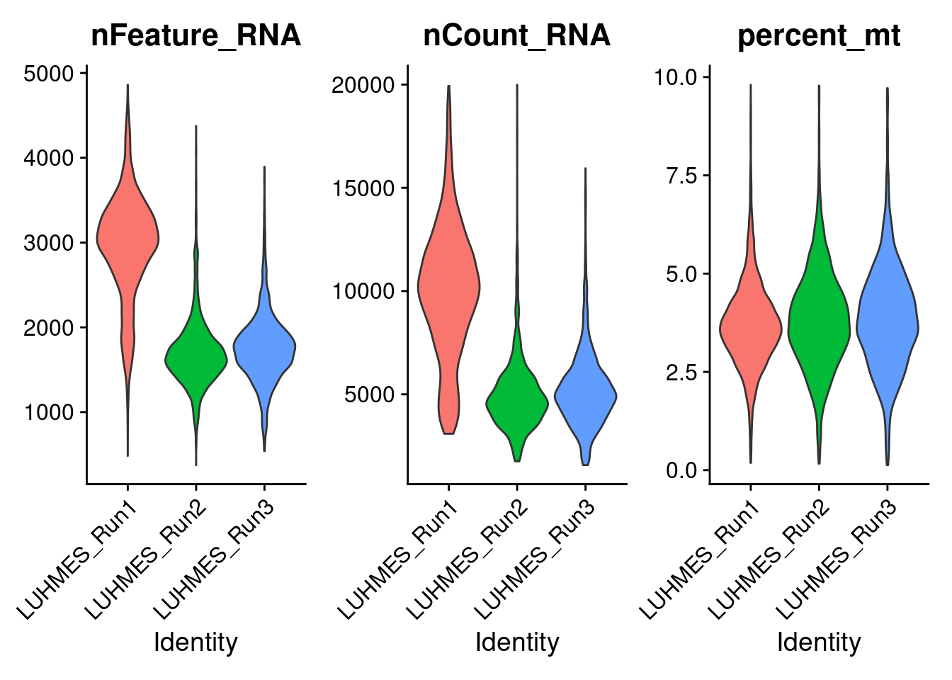
Dimensions of the merged gene expression matrix after QC:
paste0("Genes: ", dim(combined_obj)[1])
paste0("Cells: ", dim(combined_obj)[2])
[1] "Genes: 33694"
[1] "Cells: 8708"2.3 Deviance residual transformation
To accommodate the application of GSFA, we adopt the transformation proposed in Townes et al., and convert the scRNA-seq count data into deviance residuals, a continuous quantity analogous to z-scores that approximately follows a normal distribution.
The deviance residual transformation overcomes some problems of the commonly used log transformation of read counts, and has been shown to improve downstream analyses, such as feature selection and clustering.
In the following, we used the deviance_residual_transform function in GSFA to perform the tranformation.
Due to the size of the data, this process can take up to 30 minutes.
dev_res <- deviance_residual_transform(t(as.matrix(combined_obj@assays$RNA@counts)))2.4 Feature selection
Genes with constant expression across cells are not informative and will have a deviance of 0, while genes that vary across cells in expression will have a larger deviance.
Therefore, one can pick the genes with high deviance as an alternative to selecting highly variable genes, with the advantage that the selection is not sensitive to normalization.
Here we select the top 6000 genes ranked by deviance statistics, and downsize the gene expression matrix.
top_gene_index <- select_top_devres_genes(dev_res, num_top_genes = 6000)
dev_res_filtered <- dev_res[, top_gene_index]
2.5 Covariate removal
We further regressed out the differences in experimental batch, unique UMI count, library size, and percentage of mitochondrial gene expression.
covariate_df <- data.frame(batch = factor(combined_obj$orig.ident),
                           lib_size = combined_obj$nCount_RNA,
                           umi_count = combined_obj$nFeature_RNA,
                           percent_mt = combined_obj$percent_mt)
dev_res_corrected <- covariate_removal(dev_res_filtered, covariate_df)

scaled.gene_exp <- scale(dev_res_corrected)
2.6 Inputs for GSFA
The corrected and scaled gene expression matrix (8708 cells by 6000 genes) will be used as input for GSFA input argument Y. We annonate this matrix with cell and gene names so we can keep track.
sample_names <- colnames(combined_obj@assays$RNA@counts)
gene_names <- rownames(combined_obj@assays$RNA@counts)
rownames(scaled.gene_exp) <- sample_names
colnames(scaled.gene_exp) <- gene_names[top_gene_index]
In addition, we have a cell by perturbation matrix containing gene-level perturbation conditions across cells for GSFA input argument G:
G_mat <- combined_obj@meta.data[, 4:18]
G_mat <- as.matrix(G_mat)
Here is the number of cells under each gene-level perturbation:
num_cells <- colSums(G_mat)
num_cells_df <- data.frame(locus = names(num_cells),
                           count = num_cells)
ggplot(data = num_cells_df, aes(x=locus, y=count)) +
  geom_bar(stat = "identity", width = 0.6) +
  labs(x = "Perturbation",
       y = "Number of cells") +
  theme_bw() +
  theme(axis.text.x = element_text(angle = 45, hjust = 1, size =11),
        axis.text = element_text(size = 12),
        axis.title = element_text(size = 14),
        panel.grid.minor = element_blank())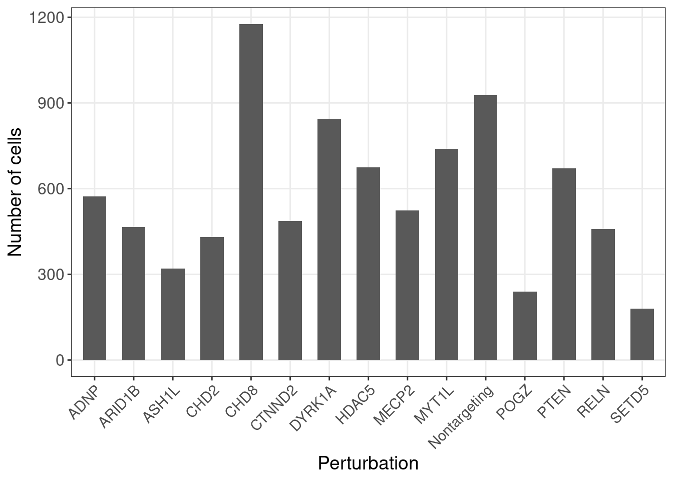
3 Session information
sessionInfo()R version 4.0.4 (2021-02-15)
Platform: x86_64-pc-linux-gnu (64-bit)
Running under: Scientific Linux 7.4 (Nitrogen)
Matrix products: default
BLAS/LAPACK: /software/openblas-0.3.13-el7-x86_64/lib/libopenblas_haswellp-r0.3.13.so
locale:
[1] LC_CTYPE=en_US.UTF-8 LC_NUMERIC=C LC_TIME=en_US.UTF-8 LC_COLLATE=en_US.UTF-8
[5] LC_MONETARY=en_US.UTF-8 LC_MESSAGES=en_US.UTF-8 LC_PAPER=en_US.UTF-8 LC_NAME=C
[9] LC_ADDRESS=C LC_TELEPHONE=C LC_MEASUREMENT=en_US.UTF-8 LC_IDENTIFICATION=C
attached base packages:
[1] grid stats graphics grDevices utils datasets methods base
other attached packages:
[1] GSFA_0.2.8 SeuratObject_4.0.0 Seurat_4.0.1 lattice_0.20-41 WebGestaltR_0.4.4 kableExtra_1.3.4
[7] ComplexHeatmap_2.6.2 gridExtra_2.3 forcats_0.5.1 stringr_1.4.0 dplyr_1.0.4 purrr_0.3.4
[13] readr_1.4.0 tidyr_1.1.2 tibble_3.0.6 ggplot2_3.3.3 tidyverse_1.3.0 Matrix_1.3-2
[19] data.table_1.14.0
loaded via a namespace (and not attached):
[1] readxl_1.3.1 backports_1.2.1 circlize_0.4.12 systemfonts_1.0.1 plyr_1.8.6
[6] igraph_1.2.6 lazyeval_0.2.2 splines_4.0.4 listenv_0.8.0 scattermore_0.7
[11] digest_0.6.27 foreach_1.5.1 htmltools_0.5.1.1 fansi_0.4.2 magrittr_2.0.1
[16] tensor_1.5 cluster_2.1.0 doParallel_1.0.16 ROCR_1.0-11 globals_0.14.0
[21] modelr_0.1.8 matrixStats_0.58.0 R.utils_2.11.0 svglite_2.0.0 spatstat.sparse_2.0-0
[26] colorspace_2.0-0 rvest_0.3.6 ggrepel_0.9.1 haven_2.3.1 xfun_0.26
[31] crayon_1.4.1 jsonlite_1.7.2 spatstat.data_2.1-0 survival_3.2-7 zoo_1.8-8
[36] iterators_1.0.13 glue_1.4.2 polyclip_1.10-0 gtable_0.3.0 webshot_0.5.2
[41] leiden_0.3.7 GetoptLong_1.0.5 future.apply_1.7.0 shape_1.4.5 BiocGenerics_0.36.1
[46] apcluster_1.4.8 abind_1.4-5 scales_1.1.1 DBI_1.1.1 rngtools_1.5
[51] miniUI_0.1.1.1 Rcpp_1.0.6 xtable_1.8-4 viridisLite_0.3.0 clue_0.3-58
[56] spatstat.core_2.0-0 reticulate_1.18 stats4_4.0.4 htmlwidgets_1.5.3 httr_1.4.2
[61] RColorBrewer_1.1-2 ellipsis_0.3.1 ica_1.0-2 pkgconfig_2.0.3 R.methodsS3_1.8.1
[66] farver_2.0.3 uwot_0.1.10 deldir_0.2-10 sass_0.3.1 dbplyr_2.1.0
[71] utf8_1.1.4 later_1.1.0.1 tidyselect_1.1.0 labeling_0.4.2 rlang_0.4.10
[76] reshape2_1.4.4 munsell_0.5.0 cellranger_1.1.0 tools_4.0.4 cli_2.3.1
[81] generics_0.1.0 broom_0.7.5 ggridges_0.5.3 fastmap_1.1.0 evaluate_0.14
[86] goftest_1.2-2 yaml_2.2.1 knitr_1.34 fs_1.5.0 fitdistrplus_1.1-3
[91] pander_0.6.4 RANN_2.6.1 nlme_3.1-152 pbapply_1.4-3 future_1.21.0
[96] doRNG_1.8.2 mime_0.10 whisker_0.4 R.oo_1.24.0 xml2_1.3.2
[101] compiler_4.0.4 rstudioapi_0.13 plotly_4.9.3 curl_4.3 png_0.1-7
[106] spatstat.utils_2.1-0 reprex_1.0.0 bslib_0.2.4 stringi_1.5.3 highr_0.8
[111] vctrs_0.3.6 pillar_1.5.0 lifecycle_1.0.0 spatstat.geom_2.0-1 lmtest_0.9-38
[116] jquerylib_0.1.3 GlobalOptions_0.1.2 RcppAnnoy_0.0.18 cowplot_1.1.1 irlba_2.3.3
[121] patchwork_1.1.1 httpuv_1.5.5 R6_2.5.0 promises_1.2.0.1 KernSmooth_2.23-18
[126] IRanges_2.24.1 parallelly_1.23.0 codetools_0.2-18 MASS_7.3-53 assertthat_0.2.1
[131] rjson_0.2.20 withr_2.4.1 sctransform_0.3.2 S4Vectors_0.28.1 mgcv_1.8-33
[136] parallel_4.0.4 hms_1.0.0 rpart_4.1-15 rmarkdown_2.11 Cairo_1.5-12.2
[141] Rtsne_0.15 shiny_1.6.0 lubridate_1.7.9.2